
- New Release! QCTool V6.5 What's new?
Summary
Download the QCTool Product Description as PDF
The essential design criteria for QCTool can be described by 3 main criteria:
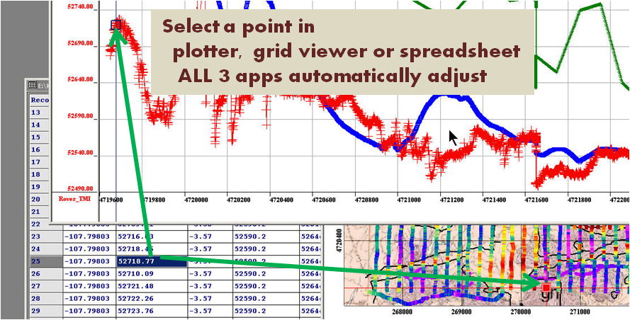
- A memory connected spreadsheet, plotter and grid display: spreadsheet functionality and information display is critical when working with data but multi-dimensional relationships are also important. The plotter provides the ability to plot channel(s)(function) versus any channel or versus the record number. But the application allows the user to naturally split their data into subsets (called lines in QCTool). The plotter plots one subset but the Grid Tool displays any channel as a function of any other 2 channels for the entire data set. The important criteria is that these three tools are fundamental to data analyses and these tools are therefore constantly linked in memory. When selecting a record in the mapped and plotted channel, this record is automatically selected in all three tools as illustrated above.
- Data compaction and Data access speed: A database typically provides data access speed while not necessarily providing a compacted data format. As the user may want to deal with millions of data points, a compact format for size is critical but also data access speeds are important. The design of using a compact, binary database type file structure gives this kind of capability and it is at the root of QCTool.
- A flexible framework for processing: By designing for digital oscilloscope type functionality, we provide the framework to easily add new processing capabilities. An individual or corporation who wishes to have a framework upon which to build specific processing may do so either by contracting us to add the processing or purchasing a developer's license to build their own tools.
Basic Functionalities
- Import
QCTool permits import of data sets no matter what size. As of now, more than 65 formats are provided: ASCII XYZ; binary XYZ; Scintrex gravity, magnetics & IP formats; Micro-g Lacoste; Geometrics magnetic formats; Geotiff; Zonge CSAMT, IP, TDEM, MT, ZEN formats; IAGA2002 Observatory data, several GEM formats; Geonics EM34/31/38, Protem and EM61 formats; GDD; GF CMD; GSSI; Garmin GDB; IRIS; Loupe; Phoenix processed data and raw time series; SeaSpy; SMARTEM; EDI formats; VLF formats; USF; SEGY; LAS; GPX; GXF; ArcGIS; BIL; Crone; GTOPO; CDED; Surpac; Geosoft formats; and others designed to meet the specific requirements of various customers. The import procedure is fully automated and easy to manage. We will happily create an import for your format.
Each data channel is kept in the storage format of your choice whether it is double or single precision (float), short or long integer, text or date or degree formats.
- Data Display
-
 Click image to enlargeGrids
There are three ways of data representation: spreadsheets, plots, and grids. All the three are interrelated and can easily be brought up for viewing at the same time. If you come across a bad-looking data in a plot, for example, you can simultaneously check it in the respective spreadsheet or grid. If you edit an erroneous data value in a spreadsheet, it is automatically adjusted in the other two applications.
- Spreadsheets
-
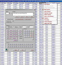 Click image to enlargeData-linked spreadsheet,
plotter and gridding
toolDepending on your choice during the import procedure, you can have your data represented as a single table of an unlimited "depth" or divide them into as many smaller tables as the number of data subsets in your original file. The links between the tables differ from those used in similar applications (e.g. Excel) due to the strict data structuring in QCTool. This feature makes it easier to work with large sets of data and saves much of your time. The spreadsheet format offers all standard functionalities usually available in similar applications.
Many processing tools are available directly from the spreadsheet. One very useful tool is the Formula Calculator that can be displayed at a click of the mouse to furnish you with the most commonly used mathematical functions from which you can develop your equations for processing. Easy access is provided to statistics and channel processing such as data sorting, interpolation, derivative calculations up to 2nd order, integrals, outlier removal and filtering.
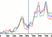
- Plots
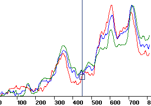
Plots are generated automatically. With them, editing data takes no time since errors are visible to the naked eye. Deleting any point on the plot will produce the same changes in the respective table or grid. You can plot as many channels as necessary to view them all at the same time; you can cut your plots into segments; switch between lines, channels, and curves; zoom in and out; change plot appearance. The plotting tool is not designed specifically for reporting purposes but for ease, speed and facility in data analyses. Several unique features are provided.
- Grids (2D Displays)
-
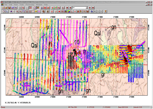
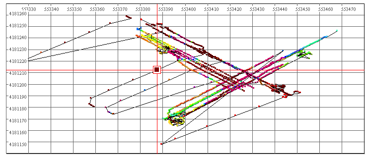
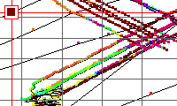 Click image to enlargeSurvey Locations
The gridding/mapping tool provides numerous convenient functionalities. You first view your lines and data points, you adjust profiles, delete points, select points for editing, apply different methods of interpolation, change draw modes, interpolate onto grids, draw and customize contours. You can also superimpose your grid or contours on a calibrated map (with calibration provided within QCTool), apply transparencies, save resulting maps.
2D data displays may be made of any column (parameter) versus any other 2 parameters quickly and easily. You may show simply the parameter at the data points (x,y), interpolate the data onto regular grids using either square or rectangular grid cells. A very accurate local interpolation technique called Natural Neighbour is allowed or the more conventional global Minimum Curvature technique. Interpolated grids may be shown as equal range (traditional) or equal area (weight). Contours may be made and filled plus many other mapping capabilities, which are integrated with 2D plot presentations.
- Mapping
QCTool is not specifically designed as a mapping software product but does provide many mapping capabilities to aid in the types of analyses which are related to maps. As well, the production of maps for reports and inclusion to other software including MapInfo, ArcMap and Google Earth is provided.
- Coordinate Transformations
Among many of the basic processing tools which are provided, various tools for manipulation of coordinates are provided. One tool is designed allowing you to convert projected (X,Y) coordinates into Latitude/Longitude in the datum of your choice and vice versa as well as conversion from one datum to another. Lambert and Polar Projections are also provided. Many ellipsoid datums are provided and if you need a different one then we can provide it. Vertical datum transformations are also now provided. Tools are also provided for manipulating time and date channels.


Additional Functionalities
- Merging Files
-
 Click image to enlarge
You may merge as many data sets as necessary and have the missing values interpolated to get the full and consistent picture of your survey. This can be done with data of different types or from different instruments but have a common data for linking such as time or date or temperature. Individual channels may be merged from one file into another.
- Append Files
You may append new data to old data. This is useful when you collect data on different days or at different times and want to bring them together.
- Generic Processing Tools
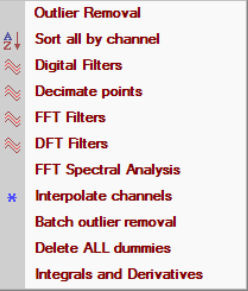
Remove outliers, sorting, a range of digital filters, data decimation, FFT and DFT spectral analyses and filtering, interpolation, first and second order derivatives, summation(integration)
- Data Shifting
If there is a lag in your data with respect to a record index, an automated function is available to shift the data channel back or forward with respect to the chosen record index. For example, if you are using a measurement system which is towed by a vehicle and the location of the data is w.r.t. to the vehicle, then the user may shift the data back along the vehicle data track. Or, if collecting data w.r.t. to time and there is a time lag or advance, then the data channel(s) can be adjusted.
- Data Stacking
Groups of records may be stacked or averaged but there is also functionality to stack the entire data array for a regular stacking or averaging. An example is if data is recorded in regular intervals and needs to be averaged or stacked through each interval
- Matrix and Vector rotations
Copyright © EiKon Technologies Ltd. 2005-2026